CHAPTER 3
The 1% —
The Pareto distribution and maximum likelihood
REFERENCE: Top Incomes in the Long Run of History»
Income inequality has been changing quite dramatically over time, in particular at the very top of the distribution, as illustrated by figure 1 on the next page, reproduced from Piketty's "Capital in the 21st century." How do we know this? In particular thanks to the careful historical work by various authors, reviewed in Atkinson et al. (2011), using tax data. In order to estimate top income shares, we need estimates of (i) how much income the rich received, and (ii) how large the total income generated in the economy was. In this chapter we shall be concerned with the question of how to get the first of these. Top incomes are estimated in this literature using historical tax data. The distribution of top incomes (and of top wealth holdings) is well approximated by the so-called Pareto distribution. The problem of estimating top incomes reduces to the problem of estimating the parameter \(\alpha\) of this distribution.
1. Definition of the Pareto distribution
We shall suppose incomes \(Y\) above an income level of \(\underline{y}\) follow a Pareto distribution. This assumption was shown to provide a good approximation in many studies. The Pareto distribution is defined by the property that
(1)
$$ P(Y>y | Y \geq \underline{y}) = \left ( \underline{y} /y\right )^{\alpha_0} $$for \(y \geq \underline{y}\), where \(\alpha_0 >1\). That is, the share of incomes above a cutoff \(y\) declines with \(y^{-\alpha_0}\). Our goal is to estimate the Pareto parameter \(\alpha_0\), which we can then use to calculate top income shares.
We can calculate the density of the Pareto distribution, conditional on \(Y \geq \underline{y}\), by taking derivatives:
(2)
$$f(Y;\alpha_0) = - \frac{\partial}{\partial y}P(Y>y | Y \geq \underline{y}) = - \frac{\partial}{\partial y} \left ( \underline{y} /y\right )^{\alpha_0} = \alpha_0 \left ( \underline{y} /y\right )^{\alpha_0}\cdot y^{-1} .$$The Pareto distribution has the interesting feature that, for any \(y\geq \underline{y}\),
(3)
$$E[Y|Y\geq y] = \frac{\alpha_0}{\alpha_0-1} \cdot y.$$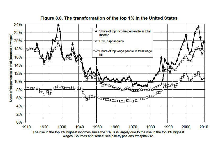
Try to verify this by calculating the expectation by integration. This equation tells us that the average income of those receiving more than \(y\), relative to \(y\), equals \({\alpha_0}/({\alpha_0-1})\) — no matter what value \(y\) we pick! The smaller the parameter \(\alpha_0\) is, the larger are the incomes received by the very rich, and the larger will be our estimates of income inequality. Suppose we know the cutoff \(q^{99}\) such that 99% of incomes are below this cutoff. We can then calculate the average income of the 1 as $$\overline{y}^{1\%} = \frac{\alpha_0}{\alpha_0-1} \cdot q^{99}.$$ You can find more information on the Pareto distribution HERE.
2. Maximum likelihood
Suppose you have i.i.d. observations \(y_1, \ldots, y_n\) of incomes above \(\underline{y}\) from historical tax data. We want to estimate the parameter \(\alpha\) using this data. One general method to construct estimators is to find the parameter which gives us the highest "probability" for finding the observations that we have; this idea is called maximum likelihood estimation (MLE). Formally, the maximum likelihood estimator is defined as(4)
$$\widehat{\alpha}^{MLE} = {\operatorname{argmax}}_\alpha \prod_{i=1}^n f(y_i; \alpha) = {\operatorname{argmax}}_\alpha \sum_{i=1}^n \log(f(y_i; \alpha)). $$This is the value of \(\alpha\) which maximizes the density of our observations. Note that between the second and third term we applied logs to everything — this is OK, since the logarithm is monotonically increasing and this therefore does not change the maximization problem.
The first order condition for the maximization problem defining the MLE (in log terms) is given by
$$ \frac{\partial}{\partial \alpha} \sum_{i=1}^n \log(f(y_i; \alpha)) = 0. $$We shall now plug in the expression for the density of the Pareto distribution which we derived before. The log likelihood of observation \(i\), that is the \(\log\) of its density given \(\alpha\), is equal to
$$\log(f(y_i; \alpha)) = \log( \alpha\left ( \underline{y} /y_i\right )^{\alpha}\cdot y_i^{-1} ) = \log( \alpha) + \alpha \log \left ( \underline{y} /y_i\right ) -\log(y_i).$$ We get $$\begin{align*} 0 &=\frac{\partial}{\partial \alpha} \sum_{i=1}^n \log( \alpha\left ( \underline{y} /y_i\right )^{\alpha}\cdot y^{-1} )\\ &= \sum_{i=1}^n \left ( \frac{1}{\alpha} + \log \left ( \underline{y} /y_i\right ) \right ) \end{align*}$$Solving for \(\alpha\) yields
(5)
$$ \begin{equation} \widehat{\alpha}^{MLE} = \frac{n}{ \sum_i \log \left (y_i/ \underline{y} \right )}. \label{eq:alphaMLE} \end{equation} $$3. Censored data
Unfortunately we usually don't observe the actual incomes that rich people received in the available tax data. All that is available from historical records is the number of tax filers that fall into several tax brackets of the form \([y_l, y_u]\). Fortunately we can still estimate the Pareto parameter from such data — which makes the Pareto distribution a very useful model. The conditional probability that \(Y\) falls in the interval \([y_l, y_u]\) can be calculated as
(6)
$$ \begin{align} P(Y \in [y_l, y_u] |Y \geq \underline{y}) &= P(Y>y_l | Y \geq \underline{y}) - P(Y>y_u | Y \geq \underline{y}) \nonumber \\ &=\left ( \underline{y} /y_l\right )^{\alpha_0} - \left ( \underline{y} /y_u\right )^{\alpha_0}. \end{align} $$For simplicity, suppose that we just observe two tax brackets, that is, we only have aggregate tax data which tell you the number \(N_1\) of taxpayers falling in the bracket \(\underline[{y}, y_l)\), and the number \(N_2\) of tax payers falling in the bracket \([y_l, \infty)\) What is the distribution of \(N_2\) conditional on \(N_1 + N_2 =n?\)
We can write \(N_2\) as a sum of independent Bernoulli random variables which take on the values 0 and 1.
$$N_2 = \sum_{i=1}^n \mathbf{1}(Y_i> y_l ),$$ where the probability that any of these variables equals \(1\) is given by $$p(\alpha_0) = P (Y> y_l | Y> \underline{y}) = \left ( \underline{y} /y_l\right )^{\alpha_0}.$$It follows that \(N_2\) is binomially distributed conditional on \(N_1+N_2=n\), that is
(7)
$$\begin{equation}N_2\sim Bin\left (n, p(\alpha_0)\right ),\end{equation}$$and
$$P(N_2 = n_2 | N_1 + N_2 =n; \alpha) = \binom{n}{n_2} \cdot p(\alpha_0)^{n_2} (1-p(\alpha_0))^{n-n_2}.$$ You can find more information on the Binomial distribution HERE.
4. Maximum likelihood with censored data
As before, we want to construct an estimator of \(\alpha_0\), but using only the interval censored data. As before, we can construct such an estimator using maximum likelihood, that is $$\widehat{\alpha}^{MLE} = {\arg\!\max}\alpha P(N_2 = n_2 | N_1 + N_2 =n; \alpha)$$ is the value which maximizes the probability of observing a number \(N_2\) of observations in the upper tax bracket.
The first order condition for the MLE is given by $$\begin{align*} 0&=\frac{\partial}{\partial \alpha} \log f(N_2|N_1+N_2; \alpha)\\ &= \frac{\partial}{\partial \alpha} \left( \log \binom{n}{N_2} + N_2 \log p + N_1 \log (1-p) \right )\\ &= \left (\frac{N_2}{p} - \frac{N_1}{1-p}\right ) \cdot \frac{\partial}{\partial \alpha} p\\ &= \left (\frac{N_2}{\left ( \underline{y} /y_l\right )^{\alpha}} - \frac{N_1}{1- \left ( \underline{y} /y_l\right )^{\alpha}}\right ) \cdot \frac{\partial}{\partial \alpha} p. \end{align*}$$
Since \(\frac{\partial}{\partial \alpha} p \neq 0\), the first term has to vanish, and after doing some algebra we see that \(\widehat{\alpha}^{MLE} \) is the solution to the equation $$\left ( \underline{y} /y_l\right )^{\widehat{\alpha}^{MLE} } = \frac{N_2}{n},$$ so that
(8)
$$\begin{equation} \widehat{\alpha}^{MLE} = \frac{\log (N_2 /n)}{\log \left ( \underline{y} /y_l\right )}. \label{eq:alphaMLEcensored} \end{equation}$$ The larger the share of our observations is that falls in the upper tax bracket, the larger is our estimate of \(\alpha\).5. Piketty's \(r-g\) and the Pareto parameter
So far, we have discussed how to estimate \(\alpha\) and how to use this estimate to calculate top income shares. But why do the top tails of income and wealth follow a Pareto distribution, and what determines the parameter \(\alpha\) One possible story is given by the formal argument underlying Piketty's book (though hidden very deeply in the references), which relates the rate of return \(r\) on capital, relative to economic growth \(g\), to the long run inequality of wealth.
I will give a heuristic proof of this argument; this is complicated and optional material. Suppose that the wealth \(Y\) of a family \(i\) follows the process
(9)
$$\begin{equation}Y_{i,1} = w_i + R_i\cdot Y_{i,0}\label{eq:wealthprocess}\end{equation}$$ over time, where \(Y_{i,1} \) denotes the wealth of children, \(Y_{i,0}\) the wealth of parents, \(w_i\) reflects savings from earnings, and \(R_i\) is the rate of savings from capital income, corresponding to Piketty's \(r-g\). Suppose further that $$(w_i, R_i) \perp Y_{i,0},$$ that is random shocks to earnings, rates of return, or savings are independent from past wealth. This is a strong assumption, which, however, could be relaxed.A so-called stationary distributionfor \(Y_i\) is one where the distribution of \(Y_{i,1}\) is the same as that for \(Y_{i,0}\) — inequality among children is the same as inequality among parents. Under fairly general conditions, this process will converge to a stationary distribution with Pareto tail as long as \(E[R] <1\) (otherwise inequality would explode over time), so that we can assume that the distribution of \(Y_0\) is already approximately Pareto in the tail of the distribution, that is for large values of wealth, $$P(Y_0>y | Y_0 \geq \underline{y}) \approx \left ( \underline{y} /y\right )^{\alpha_0}.$$
What Pareto parameter yields a stationary tail? In the tail,\(w_i\) (savings from earnings) is negligibly small relative to \(R_i \cdot Y_{i,0}\) (savings from capital income), so that stationarity requires
$$\begin{align*}
P(Y_0>y )&=P(Y_1>y ) = P(w + R\cdot Y_0>y )\\
& \approx
P(Y_0>y/R )
= E[P(Y_0>y/R | R)]
\end{align*}$$
for large \(y\), where in the second line we just dropped \(w\) from the exact equality. In the last expression we first condition on \(R\), and then average out over the distribution of \(R\).
Plugging the Pareto distribution for \(Y_0\) into these expressions we get
$$ \left ( \underline{y} /y\right )^{\alpha_0} = E\left [\left ( \underline{y} /(y/R)\right )^{\alpha_0}\right ].$$
Dividing by \(\left ( \underline{y} /y\right )^{\alpha_0}\) shows that this is equivalent to
(10)
$$ \begin{equation} E\left [R^{\alpha_0}\right ] =1. \end{equation} $$We have derived the equation mapping the distribution of \(R\) to the Pareto parameter \(\alpha_0\).
The intuition behind our argument and this equation is as follows: rich families move up the wealth distribution if their \(R_i >1\), they move down if their \(R_i<1\). Stationarity requires that upward- and downward movements cancel each other — as many families move down as up in any given range of the tail. If it's more likely to move down than up (\(R_i\) is mostly small), then there have to be fewer people that are very rich rather than just rich (large \(\alpha\), little inequality), for these movements to cancel. If it's equally likely to move up as down (\(R_i\) is centered close to \(1\)), there have to be almost as many very rich people as rich people (small \(\alpha\), lots of inequality).